3 posts tagged with "Cohort Analysis"

Introduction​

Nowadays, most applications of cohort analysis are very simple. In most cases, users are divided into different cohorts according to some attribute. For example, most papers with cohort analysis in medicine will divide patients according to their age or birthplace. Then only some simple statistical data of cohorts like average value or sum will be used. Although these are the easiest way to perform cohort analysis, they cannot provide a deeper insight into cohorts to us. We still need more effective methods.

As we have talked about in the previous blog, COOL is a cohort OLAP system specialized for cohort analysis with extremely low latency. It could process both cohort queries and OLAP queries with superb performance. With COOL, we could obtain more complex and precise cohorts. In addition, it's of great value to combine COOL with AI to dig deeper into the data.

The applications of COOL with AI​

Is the criterion for cohorts effective?​

We can evaluate the effectiveness of cohort analysis with COOL and metric learning. There are many criteria to divide the cohorts, so how to evaluate the cohorts? It's a hard problem because there are no regular distance metrics and evaluations about patients and cohorts. We could combine COOL with metric learning to find an appropriate distance metric to measure the similarities between patients. Then we could measure the cohorts with the average similarities in the same cohorts and between different cohorts. In this way, the more similar the patients in the same cohort are and the more different the patients in different cohorts are, the better the criterion is. Therefore, we could perform cohort analyses as many as we want and select the most effective criterion to dig deeper.

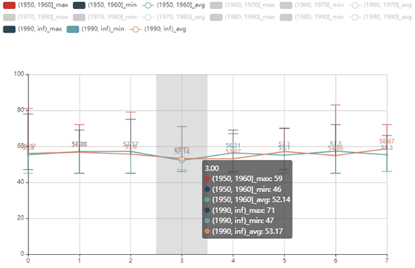
For example, we may have several assumptions to find what factors will influence mortality after admission to the ICU in 48 hours. After performing cohort analyses with COOL and viewing the maps, we find that age, score of APACHEⅡ, the time of invasive mechanical ventilation will influence the mortality. Then we can compare the effectiveness of different factors to find exactly the most important factor. We may obtain tables of similarities for different factors as follows:

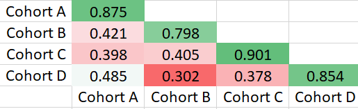
The table of similarities for age:

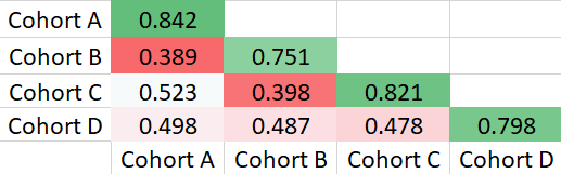
The table of similarities for score of APACHEⅡ:

The table of similarities for the time of invasive mechanical ventilation:

Finally, we can get the summary table for these factors.

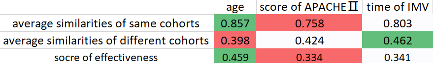
In the summary table, the score of effectiveness is defined as the difference between the average similarity of same cohorts and the average similarity of different cohorts because we hope that the patients in the same cohort are similar and the patients in different cohorts are different. Finally, we can conclude that age is the most important factor.

Process for missing values​

Estimating the missing value with COOL is an effective method and may have surprising effects. There are many missing values in big data, and we have many methods to deal with missing values, such as mean imputation, hot deck imputation and regression imputation. Now we have a new method to estimate the missing values with cohorts analysis. We could replace the missing values by averaging the corresponding values of the users in the same cohort.

For example, in a recommender system, if we consider the value to predict as the missing value, then we can extend Collaborative Filtering Approach with COOL.

In the table, users 0, 1, 2 and 3 are in the same cohort. Users 4 and 5 are in the same cohort. In general, we need to find the top k similar users to the query user and then compute the predicted value of query user. Now we can extend the method to find the top k similar users in the same cohort as the query user. Now if we want to predict the missing value of attribute_B for user 2 and set the parameter k to 2, we need to find the top 2 similar users in users 0, 1 and 3. Users 4 and 5 will not involve because they are in the different cohort from user 2.

Interpretable Features enhancement​

In some fields, such as healthcare, interpretability is of vital importance and we cannot train with uninterpretable features or models, but cohort analysis with COOL could provide interpretable cohorts or features. When the criterion of cohorts is effective, the patterns of different cohorts are different. Therefore, the representations for different cohorts are different. As a result, if we want to obtain the embeddings of users with an embedding model, it's better to train different models for different cohorts.

For example, now we have a simple approach and the structure of the method is as follows:

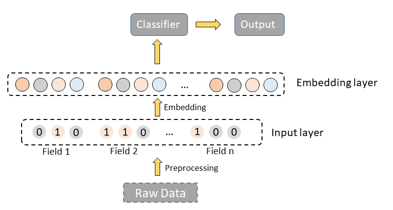
There are mainly two layers, preprocessing layer and embedding layer. Preprocessing layer is used to precess the raw data and embedding layer is to get the embedding of raw features.

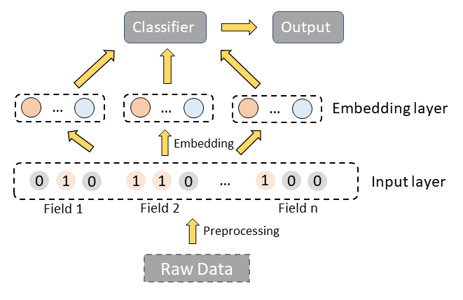
We believe the representations for different cohorts are different. So we can restructure the embedding layer and apply different embedding models to different cohorts to make the embeddings more precise and effective.

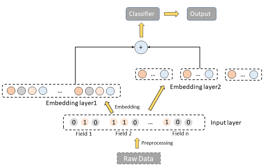
Or we can regard the new embeddings as enhanced features for raw embedding.

Conclusion​

Cohort analysis is a very effective method on top of individual analysis. Combining cohort analysis with AI will provide us with a brand new view to find more features of different cohorts. If you want to dip more into your data, have a try with COOL. The results may surprise you.

Given a set of user data for a new product, how to effectively analyze user behavior and the real user value? Conventional statistical approaches may mislead our decisions by demonstrating well-behaved average value and drawing some beautiful charts. Therefore, we are in urgent need of mastering an effective method to capture the real user value. Data never lies. However, sometimes the people who analyze the data do not do the appropriate analysis, which leads to the wrong interpretation of the user data! As an efficient data analysis method, cohort analysis is not only suitable for medical research but also of great importance for analyzing diverse groups of people in the financial area.

What is cohort analysis in finance application?​

A cohort is a subdivision of a user group, which refers to the group of users with common behavior characteristics in a specified time. Acquisition cohorts and behavioral cohorts are the two common segments, in which users are grouped by stage in the user journey and their actions in a product, respectively. Common behavioral characteristics refer to similar behaviors within a certain period, which can be categorized by different behaviors and contrasting times. For example, the users whose first purchase is in January 2021 may be grouped as a cohort. Or the frequency of use of product starts to drop in the last month of January 2021. Note that cohort analysis focuses on analyzing the differences between separate groups at the same stage of the customer life cycle.

How to Apply Cohort Analysis in Retention Analysis?​

Cohort analysis can be used in various scenarios in commercial areas, like retention analysis, churn analysis, renewal analysis, and advertising analysis. We take the retention analysis as an example to show how cohort analysis improves effectiveness for retention rate analysis.

Retention table for Product A.

Retention table for Product B.

Acquisition cohorts​

Suppose your company has two new products (Product A, Product B) released in the same period and our task is to predict which Product should be put more effort on. The user data are shown in the above two ables, which consist of the retention rate of two products in each month. The retention rate is defined as the ratio of customers who are still frequently using this product. So how to read this table? Firstly, let us look at the first row of data, in which there are 100% new registrations in the first month and about 95% of users remaining in the second month. In the third month, 3% of the users fall away. By that analogy, the number of retentions rate is about 45% in the 9th month. We can analyze the other row data in the same way. We can know the trend of retention rate for each group of newly registered users from each row. And beyond that, we can compare the retention rate of separate groups in the column domain.

In this cohort analysis example, the cohort query are:

• User selection: the users who have an account in this product;
• Birth criteria: the user is selected only if this user register an account in this product;
• Group by: the time when the user registers this account;
• Cohort matrix: the times of users' login actions in the following days.

In the first few months, the retention rate of A is higher than that of B, and the simple conclusion is that Product A is more popular than Product B. Conversely, if we take a long-term view, we find that the retention rate of Product A continues to decline, while the retention rate of Product B slowly converges to a certain value. The retention trend of an excellent product should have the following characteristics:

• The retention rate in the horizontal view should stay at a fixed value. For example, there are 100 inexperienced users in a certain month and the retention rate is stable at 50% after half a year, which means that this group of users will be valuable for the company. Otherwise, even though the retention rate declines very slowly, it may go to zero in the end. No matter how many inexperienced users there are, it is meaningless for long-term development.
• The retention data in the vertical view should be getting better. The company should constantly improve products and experiences based on users’ feedback. The users who join later should enjoy a more excellent product and service, thus leading to a higher retention rate.

But if we think a little bit more carefully. It is found that the promotion of Product A is mostly online and a small part offline, while Product B is just the opposite. Consequently, if we want to analyze the data more precisely, we need to break it down a bit more.

Behavioral cohorts​

Another popular method to group the users is based on the behaviors. For example, suppose that Product A is an APP and it has several different core features. If we want to know which core feature of APP A is of benefit to the user retention, the behavior cohort analysis can be conducted. If we measure the retention rate of Product A after users using the core feature X and core feature Y, we can learn the influence of the two core features over users' preference over this product.

Behavioral cohort analysis results for core feature X and core feature Y.

The above two tables show that the retention rate in the first table drops rapidly, which means that users does not like this core feature. Therefore, we need to improve this core feature as soon as possible. Compared### Behavioral cohorts Another popular method to group the users is based on the behaviors. For example, suppose that Product A is an APP and it has several different core features. If we want to know which core feature of APP A is of benefit to user retention, the behavior cohort analysis can be conducted. If we measure the retention rate of Product A after users use the core feature X and core feature Y, we can learn the influence of the two core features over users' preference over this product.

Behavioral cohort analysis results for core feature X and core feature Y.

The above two tables show that the retention rate in the first table drops rapidly, which means that users do not like this core feature. Therefore, we need to improve this core feature as soon as possible. Compared to the acquisition cohort, the behavioral cohort depends more on the characteristics of the product and should be able to capture more valuable user information if it is utilized effectively.

In this cohort analysis example, the cohort query are:

• User selection: the users who have registered this account in this product;
• Birth criteria: the user is selected only if this user uses the feature X at least once (times is predefined by users);
• Group by: the date when the user uses the feature X for the first time;
• Cohort matrix: the times of users' login actions in a predefined time interval.

The strength of cohort analysis is that it can not only demonstrate how people like the product but also tell us why they use or leave our product. Cohort analysis can help us to identify the merits and demerits of the product in different views, thus showing us the way to make a good product. to acquisition cohort, behavioral cohort depends more on the characteristics of the product and should be able to capture more valuable user information if it is utilized effectively.

The strength of cohort analysis is that it can not only demonstrate how people like the product but also tell us why they use or leave our product. Cohort analysis can help us to identify the merits and demerits of the product in different views, thus showing us the way to make a good product.

Introduction to COOL​

In our life, different groups of people often have different behaviors or trends. For example, the bones of older people are more porous than those of younger people, and people who exercise more are healthier than those who don't. It is of great value to explore the behaviors and trends of different groups of people, especially in healthcare, because we can adopt appropriate measures based on the behaviors and trends to make the situation better. The easiest way to do this is cohort analysis. But with a variety of big data accumulated over the years, query efficiency becomes one of the problems OnLine Analytical Processing (OLAP) systems meet, especially for cohort analysis. Therefore, COOL was designed to solve the problem.

COOL is a cohort OLAP system specialized for cohort analysis with extremely low latency.

With the support of several newly proposed operators on top of a sophisticated storage layer, COOL extends conventional OLAP systems. It could process both cohort queries and OLAP queries with superb performance.

How to perform cohort analysis with COOL?​

There are some simple concepts we need to know before performing cohort analyses.

• Birth Action: A series of actions we want to study and we need to set up the actions first.
• User Birth: A user is born when he finishes the birth actions we set up.
• Birth Time: The time when the user is born.
• Age: The age of the user is the number of time units passed since his birth.
• Metric: User-defined calculation function, such as SUM, AVERAGE and RETENTION.
• Cohort: A group of users sharing certain common characteristics when born. A user is selected into a cohort when born. We could select some features as the criterion. For example, if we select "country" as the criterion, then all the users will be selected into different country cohorts, such as the Singapore cohort, America cohort and China cohort.

Example of cohort analysis​

An example of settings of COOL is as follows:

Here, only patients diagnosed with disease B will be selected for the analysis. The birth action for patients is taking medicine A twice. The time unit of age is one day. The metric is to count patients with abnormal values in lab-test C. For each patient, the measured period, the range of the age, is the following 7 days after taking medicine A twice. Patients are selected into different cohorts according to their birth year.

Finally, we could obtain the analysis results as follows:

In the line map, each line stands for a cohort in which the patients are born in the same decade. The line map could not only illustrate the trend of patients' behavior along the time, but also offer a view of the difference between different cohorts.

The heat map is presented along with age and cohorts. Different colors give spontaneous expression on the evolvement of patient behavior and indicate deep insight into patient behavior among different cohorts.

The range map shows some statistical information of cohorts (i.e. minimum, maximum and average). The range map provides an overview of the abnormal values we want to study and a novel way to compare different cohorts and find more different features among cohorts.

From the three charts, we can observe that younger patients are easier to exhibit side effects, while elder patients take longer to get accustomed to the medicine. Most abnormal values are below 55 and few values are higher than 80. We can explore further according to the medical meaning of the values.

Conclusion​

In a word, COOL is an efficient and user-friendly cohort OLAP system specialized for cohort analysis with extremely low latency. Cohort analysis with COOL can be applied to any situation where the property of the cohort is useful to individuals and it will do good to the tasks. So why not take a look at what COOL can do for your mission?