Abstract
Designing and developing Artificial Intelligence controllers on separately dedicated chips have many advantages. This report reviews the development of a real-time fuzzy logic controller for optimizing locomotion control of a two-wheeled differential drive platform using an Arduino Uno board. Based on the Raspberry Pi board, fuzzy sets are used to optimize color recognition, enabling the color sensor to correctly recognize color at long distances, across a wide range of light intensity, and with high fault tolerance.
Keywords: fuzzy logic; fuzzy inference system; fuzzification; defuzzification; PID algorithm.
Introduction
This First Year Project (FYP) Report encapsulates my comprehensive academic journey throughout my first year at the National University of Singapore, aiming to illustrate a careful integration of concepts from modules ME3243/EE3305 Robotics System Design, EE4305 Fuzzy/Neural Systems for Intelligent Robotics, and CG2111A Engineering Principles and Practice. Through the practical application of these modules on the Arduino Uno & Raspberry Pi (RPi) robotic platform (Referred to as Robot ALEX in module CG2111A), I have engineered a rescue robot governed by fuzzy control algorithms.
In Module CG2111A, the rescue site is conceptualized as a Maze, where both the rescue robot and human operator do not have prior knowledge of the Maze's terrain. They can only identify the terrain through an onboard LiDAR system. The victim is represented by a green or red cylindrical object that can appear anywhere in the Maze. Since there are cylinders of other colors present in the Maze, the robot needs to determine the color of the cylinders to confirm whether they represent victims.
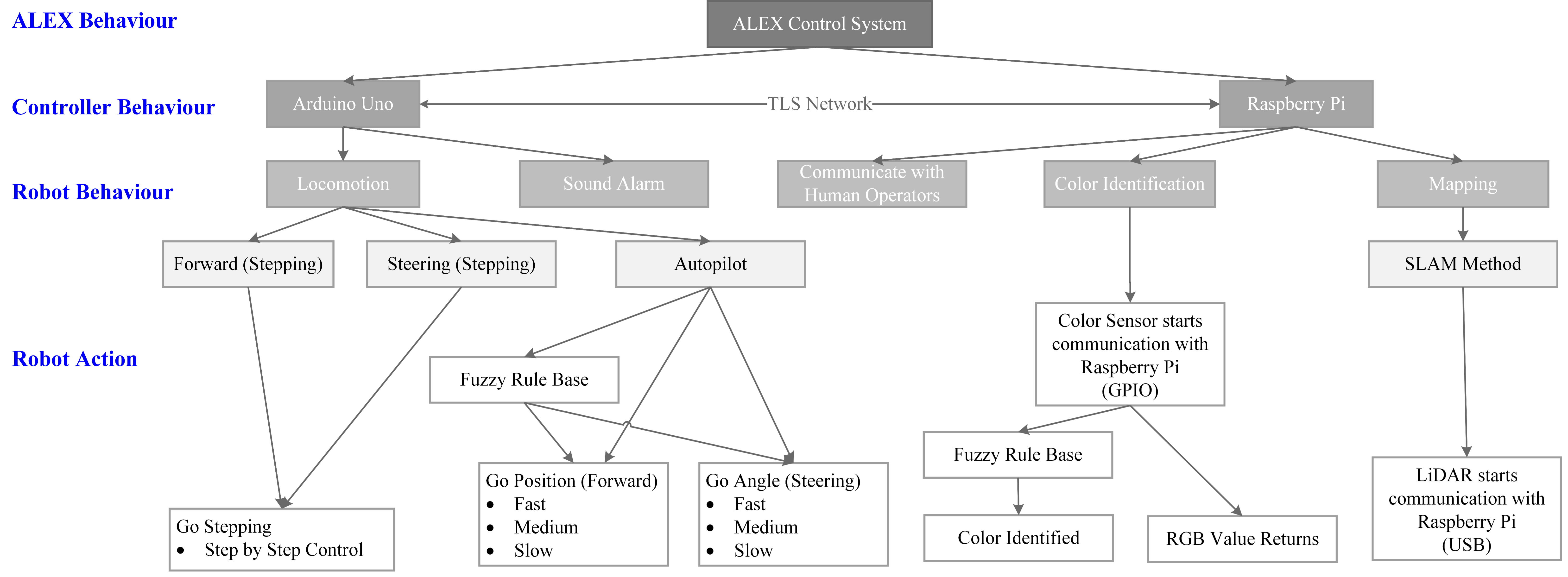
The fuzzy control algorithm optimizes the robot's locomotion and ability to identify victims. Chapters 1, 2, and 3 focus on locomotion, and Chapter 4 analyzes color recognition. Chapter 1 uses kinematic models and constraints to analyze the locomotion of the two-wheel differential drive platform, represented by the ALEX robot configuration. Chapter 2 employs the Proportional-Integral-Derivative (PID) control algorithm by using the equation of motion derived in Chapter 1 to optimize the ALEX robot's movement. Chapter 3 implements fuzzy control algorithms to refine the control accuracy of the PID algorithm. When the robot approaches a victim, it will utilize an optical color sensor to assess the victim's condition. Chapter 4 illustrates the optimization of the color-recognition process using a fuzzy algorithm. The acknowledgment, Guoyi's First Adventure in Robotics, is the final part of this paper. It will narrate my learning journey in my Year 1 at the National University of Singapore.
Chapter 1 Analysis of Locomotion
As shown in Figure 1.1, the ALEX robot controls its locomotion by adjusting the driving velocity of two active wheels on both sides. If the left and right active wheels have the same driving velocity, then the robot stays static or travels in rectilinear motion; if the left and right active wheels have different driving velocities (namely, differential velocity), then the robot performs circular motion. ALEX is a two-wheeled differential robot based on the abovementioned motion characteristics. This research only examines the motion control system of two-wheeled differential robots represented by the ALEX configuration.
 Fig 1.1 Structural diagram is the top view of ALEX. This configuration consists of a left active wheel without steering capacity, denoted by \(L\), a right active wheel \(R\), and a passive wheel. The \(O_C\) point is the robot's spin center point, which is always located at the center point of the line connecting the pivot points of the \(L\) and \(R\) wheels.
Before applying the fuzzy-PID theory to control ALEX, we first need to analyze its equation of motion to design its motion control system. The equation of motion consists of the forward equation of motion and the inverse equation of motion. The forward equation of motion calculates the movement velocity of the robot's spin center point using known driving velocities of the left and right active wheels. In contrast, the inverse equation of motion calculates the driving velocity of the left and right active wheels using the known movement velocity of the robot’s spin center point. This chapter will analyze the solutions to the forward and inverse equation of motion of ALEX. In Chapter 2, the PID control theory and the inverse equation of motion are applied to design the robot’s motion control system. Chapter 3 applies the forward equation of motion and the fuzzy control theory in tuning the motion control system.
Prior to solving the equation of motion, we need first establish the Global Reference Frame \(\xi_I\) and the Robot Local Reference Frame \(\xi_R\), as shown in Figure 1.2, to set the parameters of these equations.
 Fig 1.2 Global Reference Frame \(\xi_I\) and Robot Local Reference Frame \(\xi_R\). Angle \(\theta_I\) \((\theta_I\in{0 \leq \theta_I \leq 180^\circ})\) is the angle between the \(X_I\) axis of the \(\xi_I\) frame and the \(X_R\) axis of the \(\xi_R\) frame.
1.1 Establishing the Global Reference Frame
In the Global Reference Frame, robotic motion can be regarded as a rigid body's motion on a two-dimensional plane, which can be decomposed into a translational movement with two degrees of freedom (DOFs) and a rotary motion with one DOF. Therefore, the robotic Global Reference Frame has three theoretical degrees of freedom (DOFworkspace). The robot's locational parameters in the Global Reference Frame can be set as a vector \( \xi_I = [x_I \ y_I \ \theta_I]^T\) whose dimensions are the same as its degrees of freedom. Then, the velocity parameter of the robot in the Global Reference Frame can be set as the vector \( \dot{\xi}_I = [\dot{x}_I \ \dot{y}_I \ \dot{\theta}_I]^T\).
1.2 Establishing the Robot Local Reference Frame
The Robot Local Reference Frame \(\xi_R\) is established by taking the spin center point of the robot as the origin. To satisfy the right-hand rule, the forward motion direction of the robot is defined as the positive direction of the \(X_R\) axis, what is perpendicular to the left is the positive direction of the \(Y_R\) axis, and the \(Z_R\) axis is perpendicular to the \(O-XY\) plane to the outward direction. To sum up, the velocity parameter \( \dot{\xi}_R\)of the robot's spin center in the Global Reference Frame \(\xi_I\) can be obtained from point multiplication of the velocity vector of the Global Reference Frame \( \dot{\xi}_I\)and the orthogonal rotation matrix \( _R^IR(\theta)\):
\[
\begin{equation}
\dot{\xi}_R = I_R(\theta)\dot{\xi}_I =
\begin{bmatrix}
\cos \theta & \sin \theta & 0 \\
-\sin \theta & \cos \theta & 0 \\
0 & 0 & 1
\end{bmatrix}
\begin{bmatrix}
\dot{x}_I \\
\dot{y}_I \\
\dot{\theta}_I
\end{bmatrix}
\tag{1}
\end{equation}
\]
By now, we have already obtained the equation of motion shown in Equation (1). However, such an equation of motion contains parameters of the Global Reference Frame that the robot cannot directly obtain. Therefore, we are unable to design the robot's motion control system using Equation (1). In reality, ALEX can only control the driving velocities of left and right active wheels, namely, \(v_r\) and \(v_l\). In addition, as the active wheels of ALEX are unable to slide along the direction perpendicular to their running direction, the robot is incapable of immediately change its motion along certain directions by altering the driving velocities of active wheels. This means the robot's DOF in motion is restricted by its mechanical structure. Therefore, to determine the dimensions of the equation of motion of the robot, we need to explore the actual DOF of the moving robot equivalent to the dimensions of the equation of motion (namely, the differential degree of freedom, dDOF).
1.3 Analysis of the Dimensions of Equation of Motion
To sum up, the robot's dDOF is not equal to its DOFworkspace due to the constraint over the sliding of active wheels. The following equation can express the relationship between the constraint and DOF:
\[DOF_{workspace} = dDOF + C_f \tag{2}\]
Where \(C_f\) is the sliding constraint degree, denoting how many directions along which the active wheels are subject to sliding constraint. The active wheel coordinate frame for ALEX \(\xi_W\) is constructed, as shown in Figure 1.3.
 Fig 1.3 The Robot Local Reference Frame \( \xi_R \) and active wheel coordinate frame \( \xi_w \). Line \( E \) is set to cross the rotatory center point of active wheel \( O_w \) and is parallel to the \( X_R \) frame of the \( \xi_R \) frame. The length of the segment \( O_cO_w \) is set as \( l \), and the radius of the active wheel is set as \( r_w \). Half-line \( O_cF \) is set as the extended line of \( O_wO_c \), and half-line \( O_wG \) is perpendicular to the line \( E \). It is set that \( \angle O_wF = \angle O_wO_cX_R = \alpha \), \( \angle X_wO_wF = \beta \).
As can be known, the distance between the rotatory center point of active wheel \( O_w \) and spin center point \( O_c \) is constantly \( l \). The angle between the robot body and wheel running direction is constantly \( \alpha + \beta \). Thus, the linear velocity of active wheel \( v_w \) can be expressed by:
\[
v_w = \begin{bmatrix}
\sin(\alpha + \beta) \\
-\cos(\alpha + \beta) \\
-l\cos(\beta)
\end{bmatrix}^T
I_R(\theta)\dot{\xi}_I = r_w \cdot \omega_w \tag{3}
\]
Based on the constraints mentioned in Chapter 1.2, the normal velocity of \( v_w \) can be expressed by:
\[
\perp v_w = \begin{bmatrix}
\cos(\alpha + \beta) \\
\sin(\alpha + \beta) \\
l\sin(\beta)
\end{bmatrix}^T
I_R(\theta)\dot{\xi}_I = 0 \tag{4}
\]
As the sliding constraint capacity of the active wheel during motion only depends on wheel structure and the position where it is mounted on the robotic body, this parameter is always constant. To calculate the sliding constraint capacity of the active wheel more conveniently, we stack the reference frames of \( \xi_I \) and \( \xi_R \) to make their three axial directions align and share the same origin. At this point, the left wheel parameter is: \( \alpha_l=-\frac{\pi}{2}, \beta_l= \pi, l_l=l \) and the right wheel parameters: \( \alpha_r=\frac{\pi}{2}, \beta_r= 0, l_r=l \) then we have:
\[
\perp v_w = \begin{bmatrix}
0 & 1 & 0 \\
0 & 1 & 0
\end{bmatrix}
\begin{bmatrix}
1 & 0 & 0 \\
0 & 1 & 0 \\
0 & 0 & 1
\end{bmatrix}
\begin{bmatrix}
\dot{x}_I \\
\dot{y}_I \\
\dot{\theta}_I
\end{bmatrix}
= \begin{bmatrix}
0 \\
0
\end{bmatrix} \tag{5}
\]
So, we can get \(\dot{y}_I = 0\). This means the robot body cannot move along the direction perpendicular to the rolling direction of the active wheel, and the ALEX structured robot has one degree of sliding constraint. According to Equation (2), we get:
\[
dDOF = DOF_{workspace} - C_f = 3 - 1 = 2
\]
To sum up, the actual DOF can be determined as two by analyzing the constraint and DOF of ALEX. Hence, the equation of motion of the ALEX structured robot can be expressed as a two-dimensional vector.
1.4 Analytical Equation of Motion
The two-wheeled differential model of ALEX is shown in Figure 1.4, where the instantaneous center of rotation (\(ICR\)) is the steering center point, denoting that the robot only performs rotary motion around the point. When velocities of left and right active wheels on the same rigid body are differential, this leads to the rotation of the rigid body in motion. At this point, if the steering radius \(r_C\) is not zero, then the position of the rigid body is also changing and thus there is also translational movement. Given the sliding constraint on the robot body, the translational movement of the robot can only be fulfilled along the rolling direction of the wheel (the \(X_R\) axis direction) instead of the \(Y_R\) axis direction.
 Fig 1.4 ALEX two-wheeled differential model. The distance between \(ICR\) and \(O_C\) is set as the steering radius \(r_C\); \(L\) and \(R\) are set as the left and right active wheels of the robot, respectively; and the distance between \(L\) and \(R\) is \(d_{W}\). \(V_C\) represents the speed of the robot's center of rotation, while \(V_l\) and \(V_r\) denote the linear velocities of the left and right drive wheels, respectively.
Therefore, all points in the Robot Local Reference Frame \(\xi_R\) can be described by the angular velocity and linear velocity along the \(X_R\) axis. Based on parameters shown in Figure 1.4 and sliding constraint of ALEX derived in Chapter 1.3, the spin center point velocity can be described by the equation \(\dot{\xi}_R = [v_c \; w]^T\). As the linear velocity directions of the left and right active wheels are the same as the \(X_R\) axis and the linear velocity direction is perpendicular to steering radius, the \(ICR\) is constantly located on the connecting line between points \(L\) and \(R\), and the specific location of \(ICR\) on line \(LR\) is determined by the left and right active wheel velocity \([v_l \; v_r]\). With \(v = w \cdot r\), when \(w\) is constant, \(v\) is proportional to \(r\). Hence, the velocities of points \(L\), \(R\) and \(O_C\) can be expressed as:
\[
w = \frac{v_c}{r_c} = \frac{v_r}{r_c + \frac{d_w}{2}} = \frac{v_l}{r_c - \frac{d_w}{2}} \tag{6}
\]
Based on the formula deformation of Equation (6), the angular velocity \(w\) can be expressed as:
\[
w = \frac{v_r - v_l}{d_w} \tag{7}
\]
Further, the relationship between the linear velocity \(v_c\) of the spin center point and the left and right active wheel velocity \([v_l \; v_r]\) can be calculated by Equation (7).
\[
v_c = \frac{v_l + v_r}{2} \tag{8}
\]
1.5 Motion Equations and their Application
The Forward Motion Equation calculates the velocity of the spin center point \(O_C\) based on the velocities of the left and right driving wheels. Combining equations (7) and (8), the positive motion equation can be expressed as:
\[
\begin{bmatrix}
v_c \\
w
\end{bmatrix}
=
\begin{bmatrix}
\frac{v_r + v_l}{2} \\
\frac{v_r - v_l}{d_w}
\end{bmatrix}
=
\begin{bmatrix}
1/2 & 1/2 \\
1/d_w & -1/d_w
\end{bmatrix}
\begin{bmatrix}
v_r \\
v_l
\end{bmatrix}
\tag{9}
\]
In real-world application, encoder will be mounted on both driving wheels of the differential robot, and the linear velocities \([v_l \; v_r]\) of the two driving wheels can be calculated. At this point, the velocity of robot \(O_C\) can be calculated by Equation (9).
The Inverse Motion Equation decomposes the velocity of spin center point \(O_C\) into left and right driving wheel velocities, which can be expressed as:
\[
\begin{bmatrix}
v_r \\
v_l
\end{bmatrix}
=
\begin{bmatrix}
v_c + \frac{d_w}{2} w \\
v_c - \frac{d_w}{2} w
\end{bmatrix}
=
\begin{bmatrix}
1 & d_w/2 \\
1 & -d_w/2
\end{bmatrix}
\begin{bmatrix}
v_c \\
w
\end{bmatrix}
\tag{10}
\]
The inverse motion equation is used to control robot \(O_C\) to operate at the expected velocity \([v_c \; w]^T\), that is, the theoretical velocities of the two driving wheels are calculated by Equation (10). In the next chapter we will utilize the wheel encoder and inverse motion equation obtained in this chapter to optimize the robot's motion along the expected route in combination with the PID control theory.
Chapter 2 Implementation of PID Control Algorithm
The drive platform of the ALEX robot incorporates two DRV-8833 Motor Drivers, each equipped with an Encoder. In this chapter, we first design a PID algorithm to optimize the control of the motor, and then leverage the equation of motion that was derived in Chapter 1 to build an autopilot system to optimize ALEX's locomotion. To improve efficiency, we will initially adjust the PID parameters within the Robot Operation System (ROS) environment. Subsequently, we will conduct fine-tuning under real-world operational conditions to ensure optimal system performance and adaptability.

Fig 2.1(a) Parameters of PMDC motor
V (V): Terminal voltage of motor
I (A): Armature current
ω (rad/s): Rotational Speed
T (Nm): Torque
|

Fig 2.1(b) Characteristics Curves of motor
Speed (ω or N) - Torque (T) Curve
Current (I) - Torque (T) Curve
Power output (P) - Torque (T) Curve
Efficiency (η) - Torque (T) Curve
|
|
Source: Jones & Flynn, Mobile Robot: Inspiration to Implementation, A K Peter, 1993.
|
In actual operation, we found that the motors could not drive ALEX at low torque output, indicating that the mass of ALEX is relatively heavy compared to the torque provided by the motors. Therefore, when we change the motion state of ALEX, especially when initiating motion from a stationary state, we need to ensure that the motor can provide sufficient torque to counteract the load torque. According to the motor characteristics shown in Figure 2.1(b), this requires us to increase the input power of the motor by raising the input voltage, thereby enabling the motor to generate a larger torque and avoid stalling
When ALEX transitions from a stationary state to the desired speed, the input power is initially increased to prevent motor stalling. However, this could potentially cause ALEX to overspeed and overshoot the setpoint. This is particularly concerning because ALEX's mapping and localization, which rely on the SLAM algorithm, require the robot to move with a high degree of steadiness. Abrupt or frequent changes in motion are problematic. Therefore, it is crucial that we precisely modulate ALEX's speed. To accomplish this, we first designed a PID control algorithm for a set of motors and encoders. Then, using this initial PID control algorithm as a foundation, we designed an autopilot system to optimize the robot's motion.
2.2 PID Algorithm Enhanced PMDC Motor Control System
Figure 2.2 presents a block diagram of the PID controller in a feedback loop configuration. In this system, 'setEcd' represents the target degree of rotation of the motor, which is quantified in terms of encoder counts. 'rcdEcd' represents the current rotation of the motor. The difference between the target and the current rotation, denoted by 'errEcd' (or \( e(t) \) in Figure 2.2), is computed as the subtractive difference between 'setEcd' and 'rcdEcd'. This error value is discretely computed by the PID controller with a time difference \( t' \), which then applies a correctional factor \( u(t) \). This factor is a sum of the proportional (P), integral (I), and differential (D) terms as follows expressed mathematically with the following equation:
\[
u(t) = k_p e(t) + k_i \int_0^{t'} e(t') \, d(t') + k_d \frac{d e(t)}{d t}
\]
Term proportional (P) is the instantaneous error of the system, term integral (I) is cumulative error of the system and term differential (D) is the rate of change of error of the system.
 Fig 2.2 Block diagram of a PID controller in a feedback loop
The tuning of these PID controller parameters (\( k_p, k_i, k_d \)) is crucial as it facilitates the desired correction, thereby achieving the target motor rotation. Finally, PWM values Vpwm are generated, enabling the Arduino to regulate the speed of the PMDC motor.
2.3 PID Algorithm Enhanced Locomotion
The motion equation of ALEX analyzed in Chapter 1 and the PID Algorithm Enhanced PMDC Motor Control System designed in the previous Chapter are used to fine-tune the locomotion of ALEX.
Figure 2.3 illustrates ALEX searching for victims within a maze. The red points in the figure represent the potential locations of victims and optimal stopping points (setpoints). At each point, the robot's center of rotation \(O_C\) stops, and it can successfully complete turning or recognizing victim’s colors. Since we have requirements for the robot's orientation during turning and color recognition, we cannot make the robot move in a circular motion as shown in Figure 1.4. Moreover, when the robot moves to the setpoint, it should stop precisely at the setpoint without overshooting. To satisfy these two conditions, the optimal motion trajectory of the robot should be as shown by the gray dashed line in Figure 2.3. The robot should first rotate in place (with the ICR as the \(O_C\) point for rotation) to face the setpoint angle and then move in a straight line. Therefore, we can control the robot's turning and linear motion as two separate motion control systems – steering control system and forward control system. Decoupling these systems often leads to better stability of locomotion. It reduces the chance of instabilities that can arise from the interactions between forward and rotational motion, especially in high-speed or highly dynamic environments. For ALEX, optimal performance can be achieved by adjusting the parameters of forward and steering control system independently. For example, in a mobile robot, it might be advantageous to slow down (reduce forward speed) while turning (increasing rotational speed) to prevent tipping over.
 Fig 2.3 Orientation of ALEX in rescue environment. \(O_{LF}, O_L, O_{LB}, O_F, O_B, O_{RF}, O_R\), and \(O_{RB}\) represent the Left Front, Left, Left Back, Front, Back, Right Front, Right, Right Back setpoint respectively. \( \varphi \) is the error angle between the robot direction of motion and the setpoint.
2.3.1 Steering Control
When the robot revolves around the center of rotation \(O_C\), its linear velocity \(V_C\) should be equal to 0. Therefore, by substituting into the inverse motion equation Eq 10, we can derive the relationship between the angular velocity of rotation and the velocities of the left drive wheel \(v_l\) and the right drive wheel \(v_r\):
\[
\begin{bmatrix}
v_r \\
v_l
\end{bmatrix}
=
\begin{bmatrix}
1 & d_w/2 \\
1 & -d_w/2
\end{bmatrix}
\begin{bmatrix}
0 \\
w
\end{bmatrix}
=
\begin{bmatrix}
w \cdot d_w / 2 \\
-w \cdot d_w / 2
\end{bmatrix}
\]
Thus, the driving speeds of the left and right drive wheels are equal, but their directions are opposite. There exists the following relationship between the driving speed and the angular velocity:
\[
v = \frac{w \cdot d_w}{2}
\]
The number of rotations required for both wheels should also be equal. Therefore, after ensuring that the rotation speeds of both wheels are the same but in opposite directions, we can simply use the encoder of either the left or the right wheel to set up the PID control system.
2.3.2 Forward Control
When the robot moves in a straight line, the angular velocity \(w\) of rotation around the center point \(O_C\) should be 0. Therefore, by substituting into the inverse motion equation Eq 10, we can derive the relationship between the linear velocity of point \(O_C\) and the velocities of the left drive wheel \(v_l\) and the right drive wheel \(v_r\):
\[
\begin{bmatrix}
v_r \\
v_l
\end{bmatrix}
=
\begin{bmatrix}
1 & d_w/2 \\
1 & -d_w/2
\end{bmatrix}
\begin{bmatrix}
v_c \\
0
\end{bmatrix}
=
\begin{bmatrix}
v_c \\
v_c
\end{bmatrix}
\]
The number of rotations required for both wheels should also be equal. Therefore, after ensuring that the rotation speeds and directions of both wheels are the same, we can simply use the encoder of either the left or the right wheel to set up the PID control system.
2.4 Autopilot System
The relative distances between the robot's center of rotation (OC) and setpoints \(O_{LF}, O_L, O_{LB}, O_F, O_B, O_{RF}, O_R\), and \(O_{RB}\), along with the initial angle of motion of the robot with respect to the setpoints, are pre-stored in the program's global variables in the form of encoder counts. A human operator can command ALEX to move to any setpoints, and ALEX will engage the Steering Control and Forward Control systems to move. During this motion, ALEX utilizes an Enhanced Locomotion PID Algorithm for autonomous driving.
During Autopilot mode, the robot regularly checks if the values from the left and right encoders are equal. If the discrepancy between the encoder values exceeds a defined limit, the robot disconnects from autonomous driving and is manually taken over by the human operator.
2.5 Tuning PID Parameters in ROS Environment
To determine the optimal parameters (\(k_p, k_i, k_d\)) of PID efficiently, we migrated the parameters of the real-world environment into the ROS simulation environment. Figure 2.4 (a) and (b) respectively demonstrate the debugging of the PID parameters for the Steering Control and Forward Control systems using the ROS simulation environment.

Fig 2.4(a) Tuning Steering Controller in ROS
|

Fig 2.4(b) Tuning Forward Controller in ROS
|
2.5.1 Tuning Methods
Tuning methods are designed to tune a PID controller by adjusting \(k_p\), \(k_i\) and \(k_d\) parameters. In this project, PID controllers are tuned using a new method adapted from the Manual Tuning Method and the Ziegler–Nichols Method.
2.5.1.1 Manual Tuning Method
Manual Tuning Method is based on the effects of increasing or decreasing the gain of \(k_p\), \(k_i\) and \(k_d\) parameters separately. By analyzing the error plot curve plotted by MatPlot, Manual Tuning Method can be applied easily to tune parameters according to Table 2-1 below:
Tab 2-1 Effect of increasing the gain of any one of the parameters independently.
| Parameter Increased |
Rise Time |
Overshoot |
Settling Time |
Steady-State Error |
Stability |
| \(k_p\) |
Decrease |
Increase |
Small Change |
Decrease |
Degrade |
| \(k_i\) |
Decrease |
Increase |
Increase |
Decrease Significantly |
Degrade |
| (\(k_d\)) |
Minor Decrease |
Decrease |
Minor Decrease |
No Effect |
Improve (for small \(k_d\)) |
|
Tab 2-2 Gains for P, PI, and PID control systems
| Control Type |
\(K_p\) |
\(K_i\) |
\(K_d\) |
| P |
0.50 \(K_u\) |
- |
- |
| PI |
0.45 \(K_u\) |
1.2 \(K_p / P_u\) |
- |
| PID |
0.60 \(K_u\) |
2 \(K_p / P_u\) |
\(K_p P_u / 8\) |
|